

Apache Spark's distributed nature allows it to process massive datasets, but achieving optimal performance requires understanding its internal mechanics. When jobs crawl, fail with OutOfMemoryErrors, or show uneven task completion times, digging into data skew, memory management, shuffle behavior, and partitioning strategies is essential.

Data Skew
Data Skew originates from the combination of uneven key distribution in your data and Spark's default partitioning mechanism during shuffle operations (like join, groupByKey, reduceByKey, aggregateByKey). By default, Spark uses a HashPartitioner. For a given key, it calculates key.hashCode(), takes the modulus (%) with the number of target partitions (numPartitions), and sends all data for that key to the resulting target partition index (targetPartition = key.hashCode() % numPartitions). If one key appears far more frequently than others (e.g., a null key used as a default, or a "super-user" ID), its hash code will always map to the same target partition.
This partition becomes a bottleneck, receiving vastly more data than others. The executor processing this "heavy" partition struggles, leading to straggler tasks that dictate the overall stage completion time, even if hundreds of other tasks finish quickly. Identifying skew involves checking task metrics (duration, input size, shuffle read/write size) in the Spark UI for significant outliers within a stage.
Imagine distributing LEGO bricks into bins based on color using a simple rule: bin_number = color_code % number_of_bins. If 90% of your bricks are red (skewed key) and you have 10 bins, all red bricks will consistently hash to the same bin (e.g., red_code % 10 = bin 3). The person assigned to bin 3 (the executor task) is overwhelmed, while others with evenly distributed colors (keys) finish quickly and wait. The hashing formula (hashCode() % numPartitions) is the distribution rule, and the massive pile of red bricks in one bin is the skewed partition.
# Check key distribution before or *after shuffle operation

key_counts = df.groupBy("potentially_skewed_key").count()

# Show the most frequent keys

key_counts.orderBy(col("count").desc()).show(10)

# Analyze the distribution

key_counts.selectExpr("percentile_approx(count, 0.5)", percentile_approx(count, 0.9)", max(count)").show()
Memory Pressure
Memory Pressure occurs when Spark's memory demands exceed the allocated resources on executors or the driver. Executor memory (spark.executor.memory) is managed by the Unified Memory Manager (since Spark 1.6) and is broadly divided:
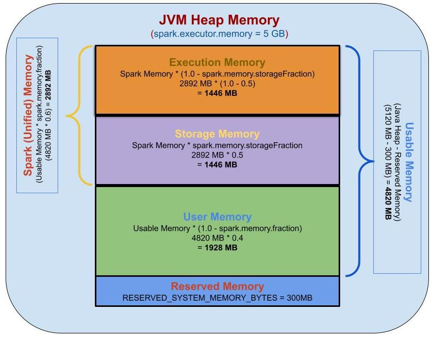
Execution Memory: Used for intermediate data during shuffles, sorts, hashes (aggregations, joins), caching data structures needed for computation. This is where most shuffle/spill issues originate.
Storage Memory: Used for caching user data.
User Memory: For UDFs, custom data structures, Spark internal metadata.
Reserved Memory: Kept aside for system overhead.
The boundary between Execution and Storage memory is flexible (spark.memory.fraction controls the combined size, spark.memory.storageFraction suggests the initial Storage portion). If Execution needs more memory, it can borrow from Storage (evicting cached blocks if necessary). If Storage needs more, it can borrow from Execution only if Execution isn't actively using it.
Pressure arises from: large deserialized objects for wide/complex rows, large shuffle blocks, aggregation buffers growing too large, insufficient total executor memory, or collecting huge results (.collect()) overwhelming driver memory (spark.driver.memory). This leads to excessive Garbage Collection (GC) – stop-the-world pauses where the JVM reclaims memory, halting task execution – and potentially Disk Spill or OOM errors.
The builder's workbench (Executor Memory) has designated areas: one for active assembly steps (Execution Memory) and one for storing pre-built sub-assemblies or commonly used parts (Storage Memory). There's also space for the instruction manual and discarded packaging (User/Reserved Memory). If a complex assembly step (shuffle/aggregation) requires laying out way more parts than fit in the assembly area, the builder might have to take apart some stored sub-assemblies (evict cached data from Storage) to make space. If even that's not enough, parts start falling off (leading to Spill or OOM). Constant pausing to frantically reorganize the messy bench is like GC.
    # Caching a very large DataFrame might fill Storage Memory

large_df.persist(StorageLevel.MEMORY_ONLY)

# Subsequent shuffles might have less Execution memory available

# Window functions over large partitions need significant buffer space

window_spec = Window.partitionBy("user_id").orderBy("timestamp")

df.withColumn("rank", rank().over(window_spec)) # Can be memory intensive per task


# Collecting a massive result to the driver

results = huge_df.limit(10000000).collect() # Driver OOM likely
Tune spark.executor.memory, spark.memory.fraction, potentially adjust partition sizes.
Disk Spill

Disk Spill is Spark's safety valve against OOM errors during memory-intensive operations within the Execution Memory region. When a task needs to allocate memory for shuffle buffers (holding data destined for other partitions), sorting data that exceeds memory, or building hash tables/buffers for aggregations, and it cannot acquire enough memory (even after potentially borrowing from Storage memory), it serializes portions of the data structure it's working on and writes it to temporary files on the executor's local disk (spark.local.dir). Later, when processing requires that spilled data, it must read it back from disk and deserialize it. This involves significant overhead: serialization/deserialization costs plus the inherent latency of disk I/O (milliseconds) compared to RAM access (nanoseconds). Even moderate spilling can drastically increase task and stage duration. It's tracked per-task and aggregated per-stage in the Spark UI ("Disk Bytes Spilled").
The builder's assembly area on the workbench (Execution Memory) is full, but they must process more bricks for the current step (e.g., sorting all blue bricks). Instead of giving up (OOM), they carefully package some already-sorted bricks into small labeled boxes (serialize) and place them neatly on the floor under the bench (spill to disk). When they later need those specific bricks, they have to find the right box, unpack it (deserialize), and bring the bricks back to the bench. This floor-retrieval process is much slower than working only on the bench.
   # Joins involving large shuffles are primary candidates

# Monitor the 'Shuffle Write Bytes' and 'Disk Bytes Spilled' during the join stage

result_df = very_large_df_1.join(very_large_df_2, "common_key")


# Grouping with a high cardinality key or large intermediate state

aggregated = big_data.groupBy("high_cardinality_key").agg(collect_list("value")) # collect_list can generate large state


# Sorting a dataset larger than available execution memory per task

sorted_df = large_df.orderBy("sort_key")
Address spill by increasing executor memory, reducing partition size (via repartition), optimizing data types, or sometimes using more memory-efficient operations.
Repartition
Repartition(numPartitions, [partitionExprs]) triggers a full shuffle operation to redistribute data into a new set of numPartitions.

Upstream Tasks: Tasks in the preceding stage read their input data partitions.
Partitioning: For each record, Spark determines its target partition in the next stage. If partition expressions (colName, expr) are provided, it computes hash(partitionExprs) % numPartitions. If no expressions are given, it assigns partitions typically in a round-robin fashion to distribute records evenly but without key locality.
Serialization & Buffering: Records are serialized and buffered in memory, grouped by target partition.
Shuffle Write: When buffers fill or the task completes, buffered data is written to shuffle files on the local disk of the current executor. These files are organized by target partition. If memory pressure exists during this write, spilling of the shuffle write buffers themselves can occur.
Network Transfer: Executors in the next stage fetch the relevant shuffle blocks (partition data) from the executors where they were written in the previous stage across the network.
Shuffle Read & Deserialization: Receiving executors read the shuffle blocks (potentially from disk if the sender spilled, or if the receiver faces memory pressure upon receiving), deserialize the data, and proceed with the next transformation or action.
Cost: This involves significant network I/O (sending data blocks between executors), disk I/O (writing/reading shuffle files, potential spill), and CPU cost (hashing, serialization/deserialization). It creates a distinct "Shuffle Boundary" (visible as a new stage) in the Spark DAG. Use it deliberately to control parallelism, break skew (round-robin or hashing on a better key), or manage output file sizes.
You have LEGOs unevenly spread across initial boxes. Repartitioning is the most thorough reorganization: every single brick is taken out (read), labeled with its destination bin number (hashing/round-robin), put into temporary transfer containers sorted by destination (shuffle write buffer/files), shipped across the room (network transfer), received by the person at the destination bin (shuffle read), unpacked (deserialize), and finally placed into the new target bins. It ensures the desired number of bins with potentially better distribution but involves handling every brick.
# Explicitly shuffle into 500 partitions using round-robin

# Good for distributing load evenly before a CPU-intensive map operation

df_even = input_df.repartition(500)


# Shuffle based on 'customer_id' into 200 partitions before joining

# Ensures all data for the same customer lands on the same partition

df_keyed = input_df.repartition(200, "customer_id")

# This join benefits from the keyed partitioning if other_df is similarly partitioned or broadcasted

result = df_keyed.join(other_df, "customer_id")


# Control output file count and potentially distribute data before write

final_df.repartition(100).write.parquet("output_path")
Coalesce

Coalesce(numPartitions) aims to reduce the number of partitions without incurring a full shuffle, making it much more efficient than repartition for this specific purpose.
Spark attempts to merge existing partitions locally. It identifies which current partitions reside on the same executor and combines them to form the new, smaller set of partitions. For instance, if you coalesce from 1000 partitions down to 100 on a 10-executor cluster, Spark might try to have each executor simply combine its local ~100 partitions into ~10 new partitions by reading the data locally and concatenating it.
Optimization: This avoids the costly network transfer and extensive disk I/O associated with a full shuffle's write/read phases most of the time. Data movement is minimized.
Limitations: It does not guarantee even data distribution in the resulting partitions. If the initial partitions being merged were already skewed, the resulting coalesced partitions will also be skewed. It cannot be used to increase the number of partitions (that requires a shuffle, use repartition).
Potential Shuffle: While highly optimized to avoid it, if the requested reduction is drastic and requires moving significant data between executors to achieve the target number, or if shuffle=True is explicitly set (df.coalesce(N, shuffle=True)), coalesce can trigger a shuffle, behaving similarly to repartition. However, the default (shuffle=False) prioritizes avoiding the shuffle.
You have 100 nearly empty small LEGO boxes scattered around (partitions after filtering). Coalescing to 10 boxes means each builder looks only at the boxes currently on their own workbench (their executor). They pick up several local boxes and simply pour their contents together into fewer, larger boxes on the same workbench. Minimal carrying across the room (network traffic) is involved. However, if one builder started with a few boxes that were much fuller than others, their final combined box might still be much fuller than boxes combined by other builders (potential imbalance).
# Assume 'filtered_df' has 1000 partitions after a filter operation

print(filtered_df.rdd.getNumPartitions()) # Output: 1000 (likely)

# Efficiently reduce partition count before writing or a small aggregation

# Much cheaper than repartition(100)

coalesced_df = filtered_df.coalesce(100)

# Check the new partition count

print(coalesced_df.rdd.getNumPartitions())

# Write fewer, larger files

coalesced_df.write.parquet("path/to/consolidated_output")
Salting

Salting directly tackles severe key skew by modifying the skewed keys to force their distribution across multiple partitions during a shuffle.
Identify Skewed Keys: Determine which keys cause the skew (e.g., via counts as shown earlier).
Augment Key: For records with skewed keys in the larger dataset, append a random "salt" value (e.g., an integer from 0 to N-1) to the original key, creating a new salted_key (e.g., originalKey_0, originalKey_1, ... originalKey_N-1). This can be done randomly for each skewed record or applied to all records for simplicity if the overhead is acceptable.
Modify Other Dataset (Joins): For the smaller dataset in a join, duplicate the rows corresponding to the skewed keys. Create N copies of each such row, appending each salt value (_0 to _N-1) to its key. Now, when the join happens on salted_key, the large dataset's skewed data is spread across N partitions, and the smaller dataset has corresponding entries in each of those partitions.
Modify Aggregation: For skewed aggregations, perform a two-stage process: first, aggregate by the salted_key. This distributes the load. Second, aggregate the results of the first stage by the original_key (stripping the salt) to get the final correct aggregate value.
Impact: Salting allows the HashPartitioner (salted_key.hashCode() % numPartitions) to distribute the previously bottlenecked data across N tasks, parallelizing the workload. The trade-off is increased data size (exploding the smaller join table) or an extra aggregation stage.
The builder with 90% of the red bricks (skewed key) is the bottleneck. Salting is like taking that red pile and randomly sticking one of 5 different labels (_A to _E) onto each red brick. Now, when hashing (label.hashCode() % numBins), "red_A" goes to bin 2, "red_B" to bin 7, "red_C" to bin 1, etc. The work is distributed across 5 bins/builders. If joining red bricks with wheel parts, you must make 5 copies of the wheel parts meant for red bricks, labeling each copy to match one salt label ("Wheels for red_A", "Wheels for red_B", etc.) so the join finds matches in all 5 bins.
from pyspark.sql.functions import (col, concat_ws, lit, rand, floor, explode,

                                   array, broadcast, monotonically_increasing_id, when)


# Assume large_df has skew on 'key', small_df is dimension table

SALT_FACTOR = 10

# Assume skewed_keys_list contains the actual keys causing skew

# skewed_keys_list = ['KEY_A', 'KEY_B'] # Example


# --- Prepare smaller DataFrame ---

# Explode only the skewed keys, keep others as is

small_df_salted = small_df.alias("s") \

    .join(broadcast(spark.range(SALT_FACTOR).toDF("salt")), how="cross") \

    .withColumn("salted_key",

        when(col("s.key").isin(skewed_keys_list), concat_ws("_", col("s.key"), col("salt")))

        .otherwise(col("s.key")) # Keep original key if not skewed

    ) \

    .select("salted_key", "s.*") # Keep original columns


# --- Prepare larger DataFrame ---

# Add salt ONLY to skewed keys to avoid unnecessary data modification

large_df_salted = large_df.withColumn("salt",

        when(col("key").isin(skewed_keys_list), floor(rand() SALT_FACTOR))

        .otherwise(lit(None)) # Or maybe lit(0) - depends on join strategy

    ) \

    .withColumn("salted_key",

        when(col("key").isin(skewed_keys_list), concat_ws("_", col("key"), col("salt")))

        .otherwise(col("key"))

    )


# --- Perform the Join ---

joined_df = large_df_salted.join(

    small_df_salted, # Broadcast potentially larger salted dimension table if possible

    "salted_key"

).drop("salt", "salted_key") # Clean up helper columns
Effectively tuning Spark requires moving beyond basic API calls and understanding the underlying data flow and resource management. Skew disrupts parallelism via uneven hashing. Memory Pressure strains executor resources, leading to GC pauses and the performance penalty of Disk Spill. Repartition offers control over parallelism and distribution via costly full shuffles, while Coalesce provides an optimized path for reducing partitions locally. Salting offers a targeted, albeit more complex, solution for severe key skew.
What to do?
Continuously monitor your jobs via the Spark UI, diagnose bottlenecks by examining task metrics and stage execution, and apply these techniques judiciously. Optimization is often an iterative process of diagnose -> tune -> measure -> repeat. Armed with this deeper understanding, you're better equipped to tame the Spark beast and achieve efficient, scalable data processing.
