Level Up Your Spark: Caching, Persistence, and Checkpointing Explained!

The Fundamentals: Cache() vs. Persist()

In Spark, caching and persisting are like having a secret weapon in your arsenal. They save the results of expensive computations (think complex RDDs or DataFrames) so you don't have to recalculate them every time you need them.

Imagine a wrestler's signature move – it's powerful but takes a lot of energy.

If they have to do it repeatedly, they'll get tired.

Caching is like having a replay ready so they don’t have to exert the energy.

cache() is like a quick mental recall of the move, while persist() is like having a video recording with different storage options.

Assuming wrestlers_df is frequently used

wrestlers_df.cache()


 Or, for more control:

from pyspark.storagelevel import StorageLevel

wrestlers_df.persist(StorageLevel.MEMORY_AND_DISK())

Storage Levels: Choosing Your Strategy

cache() uses MEMORY_ONLY by default. It's like a wrestler keeping their last move fresh in their mind.

persist() lets you choose where to store the data (memory, disk, etc.). It’s like choosing between a mental note, a detailed visualization, or a backup plan.

cache() uses MEMORY_ONLY by default

cached_wrestlers_df = wrestlers_df.cache()



 persist() requires explicit StorageLevel

from pyspark.storagelevel import StorageLevel

persisted_matches_df = matches_df.persist(StorageLevel.DISK_ONLY)

Caching for the Win: Avoiding Recomputation

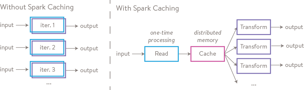
Spark uses lazy evaluation, meaning transformations only run when you trigger an action. Without caching, those transformations will re-execute every time, which can slow things down.

Think of a storyline leading up to a championship match.

Without caching, analyzing the participants would mean rewatching the entire storyline every time.

Caching is like having a summary video ready.

##### Assuming filtered_wrestlers_df is the result of a filter operation

filtered_wrestlers_df = wrestlers_df.filter(wrestlers_df["status"] == "Active")



filtered_wrestlers_df.cache() ### Cache after the filter



filtered_wrestlers_df.count() ###First action, triggers computation and caching

filtered_wrestlers_df.show() ###Second action, uses the cached data

To Cache or Not To Cache: That is the Question

Cache when you reuse data or the computation is expensive. But remember, caching uses memory. Don't cache if the data is used only once or the computation is fast. And avoid caching massive datasets that could cause memory issues.

Caching is like a wrestler perfecting a signature move they use all the time.

It's worth the effort.

But a rarely used flashy move isn't worth the practice.

And a wrestler can’t remember every past match (excessive caching).

Caching a frequently used lookup

titles_won_counts_df = wrestlers_df.groupBy("name").agg({"titles_won": "sum"})

titles_won_counts_df.cache()

titles_won_counts_df.orderBy("sum(titles_won)", ascending=False).show()

titles_won_counts_df.filter("sum(titles_won") > 5).show()

Avoiding caching a one-time use

No need to cache this if it's only used once

wrestlers_from_canada_count = wrestlers_df.filter(wrestlers_df["nationality"] == "Canada").count()

print(f"Number of Canadian wrestlers: {wrestlers_from_canada_count}")

Memory Management: The Locker Room

Spark has a reserved space in the executor JVM heap for storage. When you cache data, it goes here. Spark uses a Least Recently Used (LRU) policy to make room for new data.

The WWE locker room has limited space for gear.

Frequently needed wrestlers get priority.

If a new wrestler arrives and the room is full, those who haven't been seen lately might have their stuff moved (LRU eviction).

The management decides how much space is for gear (memory fraction).

Setting memory fraction (usually done in Spark configuration)

 This is for illustration only

 spark.conf.set("spark.memory.fraction", "0.75")  75% of heap for Spark memory

 spark.conf.set("spark.memory.storageFraction", "0.5")  50% of Spark memory for storage

Storage Levels in Detail

Here's a breakdown of the storage level options in PySpark:

MEMORY_ONLY: Stores deserialized Java objects in memory. Fastest, but memory-intensive. If memory is full, data is recomputed.

Like having a wrestler ready in the ring, but you need enough backstage space.

MEMORY_ONLY_SER: Stores serialized Java objects in memory. More space-efficient, but slower access due to deserialization. Recomputation if memory is insufficient.

Like having gear packed in bags. Less space, but need to unpack.

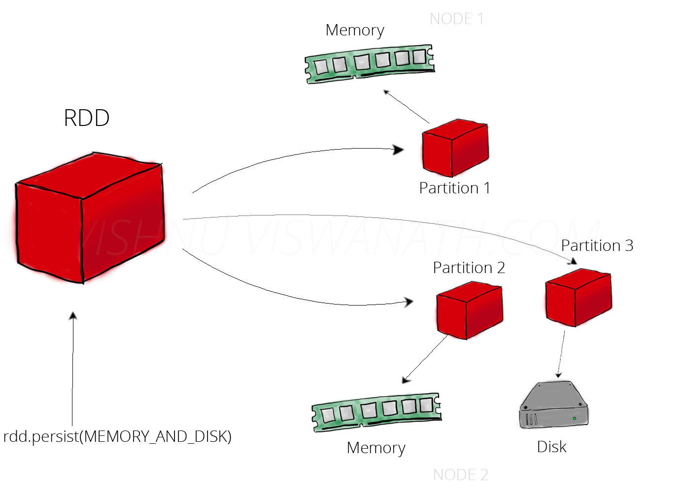
MEMORY_AND_DISK: Deserialized objects in memory, spill to disk when needed. Balances memory and performance. Disk access is slower.

Main wrestlers backstage, others in the parking lot (disk).

MEMORY_AND_DISK_SER: Serialized format with disk fallback. More space-efficient than MEMORY_AND_DISK, but requires deserialization. Disk access is slower.

Like packed bags backstage, with some in a storage unit (disk).

DISK_ONLY: Data stored only on disk. Least memory-intensive, slowest access. For very large datasets.

Match records in physical archives (disk).

OFF_HEAP: Stores serialized data in off-heap memory. Reduces JVM garbage collection overhead. Requires enabling off-heap memory in Spark configuration.

Separate storage facility outside the main arena (JVM heap).

from pyspark.storagelevel import StorageLevel


# MEMORY_ONLY

active_wrestlers_df = wrestlers_df.filter(wrestlers_df["status"] == "Active")

active_wrestlers_df.persist(StorageLevel.MEMORY_ONLY)



# MEMORY_ONLY_SER

popular_matches_df = matches_df.filter(matches_df["viewership"] > 1000000)

popular_matches_df.persist(StorageLevel.MEMORY_ONLY_SER)


# MEMORY_AND_DISK

all_match_results_df = matches_df.select("winner", "loser", "match_type")

all_match_results_df.persist(StorageLevel.MEMORY_AND_DISK)



# MEMORY_AND_DISK_SER

detailed_match_data_df = matches_df.withColumn("outcome", ...)  Some complex transformation

detailed_match_data_df.persist(StorageLevel.MEMORY_AND_DISK_SER)



# DISK_ONLY

historical_matches_df = load_very_large_dataset("historical_matches.parquet")

historical_matches_df.persist(StorageLevel.DISK_ONLY)



# OFF_HEAP (assuming off-heap memory is configured)

legacy_wrestlers_df = load_legacy_data(...)

legacy_wrestlers_df.persist(StorageLevel.OFF_HEAP)

File Formats and Caching

Let's discuss how file formats impact caching:

CSV

CSV is a row-based text format.

Parsing CSV is expensive, especially for large files.

Caching a DataFrame from CSV avoids repeated parsing.

However, CSV is less efficient for storage and queries compared to columnar formats.

Reading CSV is like reading a match transcript line by line – time-consuming.

Caching is like having a summary, but the original is still inefficient.

csv_data_df = spark.read.csv("wrestlers.csv", header=True, inferSchema=True)

csv_data_df.cache()

csv_data_df.filter(csv_data_df["weight"] > 250).count()

csv_data_df.groupBy("nationality").count().show()

Parquet

Parquet is a columnar format, optimized for analytics.

It offers better compression and faster queries than row-based formats.

Caching a Parquet DataFrame boosts performance even more.

Reading Parquet is like using a well-organized database – fast lookups.

Caching is like having the frequently used parts of the database in your working memory.

parquet_data_df = spark.read.parquet("matches.parquet")

parquet_data_df.cache()

parquet_data_df.select("winner", "match_date").show(10)

parquet_data_df.groupBy("match_type").count().show()

Compression: Parquet Crushes CSV

Parquet typically has 2-4x better compression than uncompressed CSV due to its columnar nature. Columnar storage groups similar data, enabling better compression.

CSV is like a pile of match transcripts.

Parquet is like a compressed digital archive.

Comparing file sizes

csv_data_df.write.csv("wrestlers_uncompressed.csv")

parquet_data_df.write.parquet("matches_compressed.parquet")

 Observe the file sizes on disk

Data Transfer: Efficiency Matters

Parquet's compression leads to smaller data sizes on disk and during network transfer. This means faster loading and less network usage in distributed Spark environments.

CSV transfer is like shipping a truck full of paper.

Parquet transfer is like sending a smaller digital file – faster and more efficient.

import time

start_time_parquet = time.time()

parquet_data_df = spark.read.parquet("large_matches.parquet")

end_time_parquet = time.time()

print(f"Time to read Parquet: {end_time_parquet - start_time_parquet:.2f} seconds")



start_time_csv = time.time()

csv_data_df = spark.read.csv("large_matches.csv", header=True, inferSchema=True)

end_time_csv = time.time()

print(f"Time to read CSV: {end_time_csv - start_time_csv:.2f} seconds")

When to Cache Each Format

Cache CSV when parsing is expensive and data is reused.

Like creating a reference sheet from a complex transcript.

For Parquet, caching avoids disk I/O and query execution, especially after filtering.

Like keeping your organized database readily open.

Caching after initial load for both formats if reused

csv_df_cached = spark.read.csv("frequent_data.csv", header=True, inferSchema=True).cache()

parquet_df_cached = spark.read.parquet("frequent_data.parquet").cache()

Subsequent operations on both will benefit from caching

Compression in Parquet: Getting Packed

Parquet uses various compression algorithms like Snappy, Gzip, ZSTD, and LZO. The choice depends on the balance between storage and speed.

When packing gear for travel, you can use different methods.

Snappy is like quickly folding clothes – less space, fast.

Gzip is like vacuum-sealing – much less space, more time.

ZSTD is a newer, efficient packing method.

LZO is like loosely stacking – very fast, but doesn't save much space.

matches_df.write.parquet("matches_snappy.parquet", compression="snappy")

matches_df.write.parquet("matches_gzip.parquet", compression="gzip")

matches_df.write.parquet("matches_zstd.parquet", compression="zstd")

LZO might require additional codec setup

Compression Ratio vs. Speed: A Trade-Off

Higher compression (like Gzip) takes longer to compress/decompress, while faster algorithms (like Snappy or LZO) have lower compression ratios. It's a trade-off between storage and processing speed.

Choosing compression is like deciding how much effort the backstage crew puts into packing.

Gzip is meticulous packing to save space (high compression, slower).

Snappy is a quicker pack, saving some space without much delay (moderate compression and speed).

import time

start_time_snappy = time.time()

spark.read.parquet("matches_snappy.parquet").count()

end_time_snappy = time.time()

print(f"Time to read Snappy compressed Parquet: {end_time_snappy - start_time_snappy:.2f} seconds")



start_time_gzip = time.time()

spark.read.parquet("matches_gzip.parquet").count()

end_time_gzip = time.time()

print(f"Time to read Gzip compressed Parquet: {end_time_gzip - start_time_gzip:.2f} seconds")

Columnar Storage: Compression Champion

Parquet's columnar format enables better compression. Data within a column is similar, so compression algorithms work more efficiently.

Imagine sorting gear by type: all boots together, all belts together (columnar).

This is easier to compress than a random mix (row-based).

Parquet's columnar nature automatically helps in better compression

matches_df.write.parquet("matches_compressed.parquet")

Type-Specific Encoding: Extra Efficiency

Parquet uses type-specific encoding schemes within columns. These encodings are optimized for the column's data type (e.g., dictionary encoding, delta encoding), further reducing storage.

Beyond packing, Parquet uses special ways to represent gear.

It might use a code for "WWE Championship" instead of writing it out repeatedly (dictionary encoding).

For weights, it might store the difference from the previous weight (delta encoding).

Spark handles these encodings automatically when writing Parquet

Spark automatically applies appropriate encoding schemes

wrestlers_df.write.parquet("wrestlers_encoded.parquet")

Network Transfer: Smaller is Faster

Compression in Parquet means smaller file sizes, leading to more efficient network transfers in Spark. Less data means faster movement and lower network usage.

Transferring compressed Parquet is like shipping lighter boxes.

It takes less time and fuel (network bandwidth).

In a distributed Spark setup, reading and writing compressed Parquet will generally result in less network traffic and faster operations

aggregated_data = matches_df.groupBy("event").count()

aggregated_data.write.parquet("event_counts_compressed.parquet", compression="snappy")

 Later, reading this data across the cluster will be more efficient

loaded_counts = spark.read.parquet("event_counts_compressed.parquet")

Performance Benchmarking: Let's Get Ready to Rumble!

Read/Write Performance

Read: Parquet is generally faster, especially for analytical queries that use only some columns. CSV requires reading the whole row.

Getting wrestler statistics is faster from Parquet (columnar) than CSV transcripts (row-based).

Write: Parquet write times vary by compression. Highly compressed Parquet might be slower than CSV. But Parquet's benefits often outweigh this.

Recording match results might be slower in Parquet if you're organizing and compressing, but the long-term benefits are worth it.

import time

 Assuming large CSV and Parquet files exist

start_time_parquet_read = time.time()

spark.read.parquet("large_matches.parquet").select("winner").count()

end_time_parquet_read = time.time()

print(f"Time to read 'winner' column from Parquet: {end_time_parquet_read - start_time_parquet_read:.2f} seconds")



start_time_csv_read = time.time()

spark.read.csv("large_matches.csv", header=True, inferSchema=True).select("winner").count()

end_time_csv_read = time.time()

print(f"Time to read 'winner' column from CSV: {end_time_csv_read - start_time_csv_read:.2f} seconds")



start_time_parquet_write = time.time()

matches_df.write.parquet("temp_parquet.parquet", compression="snappy")

end_time_parquet_write = time.time()

print(f"Time to write Parquet: {end_time_parquet_write - start_time_parquet_write:.2f} seconds")



start_time_csv_write = time.time()

matches_df.write.csv("temp_csv.csv")

end_time_csv_write = time.time()

print(f"Time to write CSV: {end_time_csv_write - start_time_csv_write:.2f} seconds")

Caching and Query Performance: A Tag Team

Caching greatly improves performance for repeated queries on the same data by avoiding disk I/O and recomputation. The more expensive the initial computation, the bigger the gain.

Once you have a mental scorecard of wrestlers, you can quickly answer questions without rewatching old matches.

expensive_computation_df = matches_df.groupBy("event", "match_type").agg({"viewership": "avg", "attendance": "avg"})

expensive_computation_df.cache()   Cache the result



start_time_query1 = time.time()

expensive_computation_df.filter(expensive_computation_df["avg(viewership)"] > 500000).count()

end_time_query1 = time.time()

print(f"Time for first query (after caching): {end_time_query1 - start_time_query1:.2f} seconds")



start_time_query2 = time.time()

expensive_computation_df.filter(expensive_computation_df["avg(attendance)"] > 10000).show()

end_time_query2 = time.time()

print(f"Time for second query (using cached data): {end_time_query2 - start_time_query1:.2f} seconds")



expensive_computation_df.unpersist()

Memory Usage: How Much Space Do They Need?

In deserialized form (MEMORY_ONLY), CSV and Parquet memory usage might be similar.

But in serialized forms (MEMORY_ONLY_SER, MEMORY_AND_DISK_SER), Parquet, often already compressed, can use less memory than CSV.

Think of storing wrestler info. Parquet can store metadata more efficiently.

When you pack it away (serialize), Parquet might take up less space in your "locker" (memory).

Observing Spark UI's "Storage" tab after caching can give insights

csv_data_df = spark.read.csv("large_wrestlers.csv", header=True, inferSchema=True).cache()

parquet_data_df = spark.read.parquet("large_matches.parquet").cache()

 Check the Spark UI to see the memory size of each DataFrame

csv_data_df.unpersist()

parquet_data_df.unpersist()

Comparative Metrics: 10 Million Row Datasets

With a 10M row dataset:

Storage size: Parquet (with compression) will be much smaller than CSV.

Read time (cold cache): Parquet can be faster, especially for column selection. CSV read time is mostly parsing.

Read time (warm cache): Both will be very fast if fully cached.

Query time (after caching): Similar, but Parquet can still be better for some queries (e.g., aggregations).

Memory footprint (cached): Parquet might use less memory in serialized form.

Managing data for 10 million fans: Parquet is like an optimized database, CSV is like a massive spreadsheet. Caching speeds up access, but Parquet is more efficient.

This is a conceptual example, you'd need to generate or load a 10M row dataset

large_wrestlers_csv = spark.read.csv("large_10m_wrestlers.csv", header=True, inferSchema=True)

large_matches_parquet = spark.read.parquet("large_10m_matches.parquet")



start_time = time.time()

large_wrestlers_csv.filter(large_wrestlers_csv["weight"] > 200).count()

end_time = time.time()

print(f"Time to filter CSV (cold): {end_time - start_time:.2f} seconds")



large_wrestlers_csv.cache()

start_time = time.time()

large_wrestlers_csv.filter(large_wrestlers_csv["weight"] > 200).count()

end_time = time.time()

print(f"Time to filter CSV (warm): {end_time - start_time:.2f} seconds")



start_time = time.time()

large_matches_parquet.filter(large_matches_parquet["viewership"] > 100000).count()

end_time = time.time()

print(f"Time to filter Parquet (cold): {end_time - start_time:.2f} seconds")



large_matches_parquet.cache()

start_time = time.time()

large_matches_parquet.filter(large_matches_parquet["viewership"] > 100000).count()

end_time = time.time()

print(f"Time to filter Parquet (warm): {end_time - start_time:.2f} seconds")



large_wrestlers_csv.unpersist()

large_matches_parquet.unpersist()

Filter and Aggregation: Parquet's Power Plays

Filtering: Parquet uses predicate pushdown, applying filters early to reduce the data read and processed. This is faster than CSV.

When finding wrestlers by weight, Parquet can scan the weight column directly (predicate pushdown). CSV has to read every record.

Aggregation: Parquet only reads the necessary columns for aggregations, improving efficiency.

To calculate average titles won, Parquet only reads the "titles_won" column. CSV reads entire rows.

start_time_parquet_filter = time.time()

parquet_data_df.filter(parquet_data_df["weight"] > 250).count()

end_time_parquet_filter = time.time()

print(f"Time to filter Parquet: {end_time_parquet_filter - start_time_parquet_filter:.2f} seconds")



start_time_csv_filter = time.time()

csv_data_df.filter(csv_data_df["weight"] > 250).count()

end_time_csv_filter = time.time()

print(f"Time to filter CSV: {end_time_csv_filter - start_time_csv_filter:.2f} seconds")



start_time_parquet_agg = time.time()

parquet_data_df.groupBy("nationality").agg({"titles_won": "avg"}).show()

end_time_parquet_agg = time.time()

print(f"Time to aggregate Parquet: {end_time_parquet_agg - start_time_parquet_agg:.2f} seconds")



start_time_csv_agg = time.time()

csv_data_df.groupBy("nationality").agg({"titles_won": "avg"}).show()

end_time_csv_agg = time.time()

print(f"Time to aggregate CSV: {end_time_csv_agg - start_time_csv_agg:.2f} seconds")

Monitoring and Management: Backstage Control

Spark UI: Your Control Room

The Spark UI provides information about cached RDDs/DataFrames. The "Storage" tab shows what's cached, storage level, partitions, size, and where it's stored.

The Spark UI is like the backstage control room.

The "Storage" tab shows which wrestlers are ready, what gear they have, where they are, and if anyone is in overflow storage (disk).

Access the Spark UI (usually http://<driver-node>:4040)

Navigate to the "Storage" tab to view cached data.

Checking Cache Status and Memory Usage

is_cached checks if an RDD/DataFrame is cached.

getStorageLevel() gets the storage level of an RDD.

Detailed memory usage is in the Spark UI or monitoring systems.

is_cached is like asking if a wrestler is backstage.

getStorageLevel() is like checking their preparation (warmed up, geared up, or in storage).

Detailed information is in performance reports (Spark UI).

cached_wrestlers_df = wrestlers_df.cache()

print(f"Is wrestlers_df cached? {cached_wrestlers_df.is_cached}")



from pyspark.storagelevel import StorageLevel

persisted_matches_rdd = matches_df.rdd.persist(StorageLevel.MEMORY_AND_DISK_SER)

print(f"Storage level of matches_rdd: {persisted_matches_rdd.getStorageLevel()}")

More detailed memory usage typically inspected via Spark UI

Preventing Excessive Caching: Use What You Need

Only cache data that is reused and provides a performance benefit. Be mindful of memory. Unpersist data you don't need anymore.

Don't bring every piece of gear to every event (excessive caching).

Only bring what you need.

Put gear back in storage (unpersist) to free up space.

frequently_used_df = wrestlers_df.filter(wrestlers_df["status"] == "Active").cache()

... perform operations using frequently_used_df



frequently_used_df.unpersist()   Remove from cache when no longer needed



intermediate_result_df = some_transformation(data_df)

 Use intermediate_result_df

final_result_df = another_transformation(intermediate_result_df)

 No need to cache intermediate_result_df if it's not used again

Memory Pressure: Too Many Wrestlers Backstage

Monitor memory usage in the Spark UI. If you have memory pressure (e.g., garbage collection, disk spilling), you can:

Reduce cached RDDs/DataFrames.

Use a less memory-intensive storage level (e.g., MEMORY_ONLY_SER).

Increase executor memory (if possible).

Optimize data processing to hold less data in memory.

If the backstage is crowded, some wrestlers can wait in overflow (disk spilling), some can pack more efficiently (serialized storage), or you need a bigger backstage (increase memory).

You might need to streamline the match schedule (optimize processing).

Unpersist less critical cached data

less_important_df.unpersist()



 Persist with a less memory-intensive storage level

large_df.persist(StorageLevel.MEMORY_AND_DISK_SER)



 Consider increasing executor memory in Spark configuration

 spark-submit --executor-memory 4g ...



 Optimize transformations to process data in smaller chunks if possible

Tracking Cached Data: Keep an Eye on the Roster

Use descriptive names for DataFrames/RDDs to find them easily in the Spark UI.

Know which data structures are cached.

Check the Spark UI to ensure caching is effective and not causing issues.

Give each wrestler and their gear clear labels (descriptive names) so the crew can track them.

Have a mental checklist of who is backstage.

Review the monitor to ensure everything is organized.

active_wrestlers_cached_df = wrestlers_df.filter(wrestlers_df["status"] == "Active").cache()

main_events_matches_persisted_df = matches_df.filter(matches_df["match_type"] == "Main Event").persist(StorageLevel.MEMORY_AND_DISK())

Caching Best Practices: Strategies for Success

Frequently Accessed Views: Your Go-To Moves

Identify DataFrames/RDDs used repeatedly (e.g., intermediate results, lookup tables).

Cache these "views" to avoid recomputation.

Choose the right storage level based on size and access frequency.

Identify your signature moves (frequently accessed views).

Have them ready (cached) so you don't have to figure them out every time.

Choose the best way to remember them (storage level).

Create a frequently used lookup of wrestler names to their weight

wrestler_weight_lookup_df = wrestlers_df.select("name", "weight").cache()

 Use this lookup in multiple subsequent operations

heavyweight_matches_df = matches_df.join(wrestler_weight_lookup_df, matches_df["winner"] == wrestler_weight_lookup_df["name"]).filter(wrestler_weight_lookup_df["weight"] > 250)

... another join or filter using wrestler_weight_lookup_df ...

Transformations Before Caching: Filter First

Apply filtering and projection before caching if they reduce the data size. Caching a smaller dataset is more memory-efficient. Don't cache raw data if only a subset is used.

Before memorizing a sequence (caching), filter out unnecessary moves (apply filters/projections).

Don't remember the entire match if you only need segments.


 Filter for main event matches before caching

main_event_data_df = matches_df.filter(matches_df["match_type"] == "Main Event").cache()



 Select only relevant columns before caching

wrestler_names_nationalities_df = wrestlers_df.select("name", "nationality").cache()

Choosing Storage Levels: Match the Roster Size

Small datasets: MEMORY_ONLY or MEMORY_ONLY_SER for fast access.

Larger datasets: MEMORY_AND_DISK or MEMORY_AND_DISK_SER to use disk.

Very large datasets: DISK_ONLY if memory is limited (slower).

For reducing GC overhead: Explore OFF_HEAP.

Small group of key wrestlers: Keep them ready (MEMORY_ONLY).

Larger roster: Main wrestlers backstage, others on standby (MEMORY_AND_DISK).

Massive roster: Records in the archive (DISK_ONLY).

Long event with a huge roster: External staging area (OFF_HEAP).

Lazy Evaluation and Caching: Time Your Move

cache() and persist() are lazy. Caching happens when an action is performed for the first time after calling them. Plan your caching so data is cached right before it's used in multiple actions.

Don't start practicing a move too early if you won't use it for a while.

Wait until you're about to use it multiple times.

transformed_df = data_df.filter(...).groupBy(...).agg(...)

transformed_df.cache()   Cache right before the first action that uses it heavily

transformed_df.count()   First action triggers caching

transformed_df.show()    Subsequent action uses the cached data

Removing Cached Data: Clean Up the Locker Room

Use unpersist() to remove an RDD or DataFrame from the cache.

Use spark.catalog.clearCache() to remove all cached tables and DataFrames.

Use with caution!

cached_df = some_df.cache()

... use cached_df ...

cached_df.unpersist()

 To clear all cached tables and DataFrames:

 spark.catalog.clearCache()

Level Up Your Caching Game

Caching in Spark SQL: Management's Decisions

Spark SQL manages caching for tables and views. Use spark.catalog.cacheTable("tableName") to cache a table. Spark SQL's Catalyst optimizer can also cache intermediate results. Use spark.catalog.isCached("tableName") to check if a table is cached. The default storage level is MEMORY_AND_DISK.

Spark SQL is like management that can "feature" wrestlers/storylines (cache tables/views).

They have strategies to optimize events (Catalyst optimizer, implicit caching).

You can check the official roster (isCached) to see who is featured.

matches_df.createOrReplaceTempView("matches_view")

spark.catalog.cacheTable("matches_view")

print(f"Is matches_view cached? {spark.catalog.isCached('matches_view')}")



 To uncache:

 spark.catalog.uncacheTable("matches_view")

 spark.catalog.clearCache()   Clears all



 You can also cache a DataFrame directly as a table

wrestlers_df.write.saveAsTable("wrestlers_table")   Creates a managed table

spark.catalog.cacheTable("wrestlers_table")

Cache Partitioning: Grouping the Wrestlers

The number of partitions in a cached RDD/DataFrame affects performance. Too few partitions underutilize executors, while too many small partitions increase overhead. Ideally, the number of partitions should be a multiple of the number of cores. The partitioning before caching influences the cached data. You might need to repartition before caching.

Partitions are like groups of wrestlers backstage.

Too few groups: Some groups are too large.

Too many small groups: Organizers spend too much time coordinating.

Ideally, you want balanced groups that align with dressing rooms (cores).

The initial organization (partitioning before caching) affects the backstage groups.

You might need to reorganize them (repartition before caching).

Check the number of partitions

print(f"Number of partitions before repartition: {matches_df.rdd.getNumPartitions()}")



 Repartition to a more suitable number (e.g., 4 times the number of cores)

repartitioned_df = matches_df.repartition(16)   Assuming 4 cores  4

repartitioned_df.cache()

print(f"Number of partitions after repartition and cache: {repartitioned_df.rdd.getNumPartitions()}")

Fault Tolerance: Backup Plans

Caching improves performance but can introduce a failure point. If an executor with cached data fails, the data might be lost. Spark can recompute it, but this takes time. Disk-based storage levels (MEMORY_AND_DISK, DISK_ONLY) are more fault-tolerant than MEMORY_ONLY. Replication (e.g., MEMORY_ONLY_2) further enhances fault tolerance but uses more storage.

A wrestler relying on memory (MEMORY_ONLY) might lose it if they get "knocked out" (executor failure).

A backup plan (MEMORY_AND_DISK) provides a reference.

Multiple wrestlers knowing the same move (replication) ensures it can still be performed.

For performance-critical but potentially lossy caching

performance_df.persist(StorageLevel.MEMORY_ONLY)



 For better fault tolerance, even with some performance overhead

resilient_df.persist(StorageLevel.MEMORY_AND_DISK)



 For high fault tolerance (replication), if needed and configured

from pyspark.storagelevel import StorageLevel

replicated_df.persist(StorageLevel.MEMORY_ONLY_2)

Spark Job Scheduling: Location, Location, Location

Caching influences Spark job scheduling. Spark tries to schedule tasks on executors where the data is cached (data locality). This reduces network transfer and speeds up job completion. Effective caching improves data locality and job efficiency.

If a wrestler needs equipment (cached data), it's better if it's already in their location (executor).

The organizers (Spark scheduler) will try to assign them to a ring (executor) where the equipment is ready, avoiding transport (network transfer).

The benefit is largely automatic through Spark's scheduling

cached_data = some_expensive_operation().cache()

 Subsequent actions on cached_data will benefit from data locality

result1 = cached_data.map(...)

result1.count()   Tasks will ideally run on executors with cached_data

result2 = cached_data.filter(...)

result2.show()    More tasks will benefit from data locality

Broadcast Variables vs. Cached DataFrames: Sharing the Knowledge

Broadcast variables and cached DataFrames both reduce data transfer. Broadcast variables share small, read-only datasets across executors. Cached DataFrames are for larger, reused datasets. Broadcast variables are copied to each executor, while cached DataFrames are partitioned and stored across executors. The choice depends on the dataset size and how it's used.

Broadcast Variables: Like a small playbook of key strategies that every wrestler carries.

It's small and easily distributed.

Cached DataFrames: Like a larger database of opponent statistics at each training facility (executor).

It's too big for everyone, but readily available.

Broadcast variable for a small lookup table

country_codes = {"USA": 1, "Canada": 2, "Mexico": 3}

broadcast_country_codes = spark.sparkContext.broadcast(country_codes)

mapped_rdd = wrestlers_df.rdd.map(lambda row: (row.name, broadcast_country_codes.value.get(row.nationality)))



 Cached DataFrame for a larger, frequently used dataset

frequent_data_df = large_dataset.filter(...).cache()

joined_df = another_df.join(frequent_data_df, ...)

Checkpointing: Saving the Key Moments

Checkpointing saves intermediate results to stable storage (e.g., HDFS) to break long RDD lineages. This improves fault tolerance and reduces lineage tracking overhead.

Like saving a key match moment on video.

If something goes wrong, you restart from that point, not the beginning.

sc.setCheckpointDir("hdfs:///tmp/checkpoints")

filtered_data.checkpoint()

print(filtered_data.collect())

When to Use Checkpointing: Save the Big Events

Use for long, expensive lineages or iterative jobs where recomputation is costly and fault tolerance is important. Avoid for short lineages or frequent, small computations due to I/O overhead.

Save major title changes or turning points, not every minor promo.

Triggering Checkpointing: Action!

rdd.checkpoint() marks for checkpointing. The actual saving happens on the next action. Force immediate checkpointing with an action like count() after checkpoint().

Saying a moment is a "checkpoint" vs. the cameras actually recording it.

checkpointed_rdd.checkpoint()

checkpointed_rdd.count()

Storage Levels and Checkpointing: Teamwork

Persistence (cache/persist) is for performance within a job. Checkpointing is for fault tolerance across jobs/failures. Use both: persist for speed, checkpoint for resilience.

Keeping strategy notes handy (persist) vs. having official match recordings (checkpoint) for reliability.

iterative_data = iterative_data.persist(StorageLevel.MEMORY_ONLY)

iterative_data.checkpoint()

iterative_data.count()

Lineage Truncation and DAG Size: Simplifying the Story

Checkpointing reduces the length of the RDD lineage graph (DAG), making it more manageable and improving recovery time.

Simplifying a long storyline by creating a new "current state" at a major event.

Overhead of Checkpointing: Use Wisely

Checkpointing has I/O cost due to writing to stable storage. Use judiciously for critical RDDs with long lineages where fault tolerance outweighs the cost.

Saving every detail disrupts the show; save only the important moments.